Study of the impact of climate change on the runoff of the Varzob River Basin in Tajikistan

1. Introduction

Climate change is affecting Central Asia in multiple ways, namely changes in air temperature, amount of precipitation, and water balance. Studies conducted by Li et al. (2024) and Yao et al. (2024) indicated that the year 2024 had the warmest temperature in the recorded history. The typical arid and semiarid terrain of Central Asia is tremendously vulnerable to changes in climate (Hu et al., 2014). “Climate change alters hydrological cycles and streamflow regimes at the local, regional and global levels” (Ich et al., 2022). These changes can influence the amount of water in rivers, potentially resulting in flooding, drought, and water security challenges. Additionally, there is a likely increase in the risk of spring flooding as well as glacial lake outbursts during snowmelt due to the quantity of meltwater exceeding its historical level (Profile, 2010). Several studies have investigated climate change in Central Asia over different periods. From 1942 to 2003, Feng et al. (2018) observed a temperature increase of 0.65°C, and they predicted further warming in the coming decades (Mannig et al., 2013). Another study projected a more severe scenario, with a potential 7°C rise in mean temperature by the end of the 21st century (Mannig et al. 2013). Multiple other studies highlight that if temperatures exceed 1.5°C of warming this could have detrimental effects on world net primary food production (Pan et al., 2014, Zhang & Ren, 2017). Klein Tank et al. (2006) found that between 1961 and 2000, both cold and warm extreme temperatures increased in Central and South Asia. As for precipitation, historical data showed a slight increase in the mountains of Uzbekistan, northern Kyrgyzstan, and central Tajikistan (western Pamir and Turkestan-Alai), while a decrease in precipitation was observed in southern and eastern parts of Turkmenistan, Kazakhstan, Tajikistan (particularly in the eastern Pamirs), and the central Tien Shan of Kyrgyzstan (Christiane et al., 2009). Similarly, other studies indicated an increase in precipitation in Central Asia's dry region from 1930 to 2009 (Chen et al., 2012). One study analyzed data from 1891 to 2011 and found a significant upward trend in annual precipitation (4.44 mm per decade) in the Syr Darya Basin (Yao & Chen, 2015). It is worth noting that precipitation patterns varied across seasons, as reported by earlier research (Maillard et al., 2018).

In recent years, due to climate change, water security and particularly the water supply of the urban population not only in Tajikistan but also around the world is becoming one of the most critical problems (Gulayozov & Fazylov, 2022a). Recent reports and simulation studies predict adverse effects on the global yields of all major crops due to climate change (Liu et al., 2020). The main water artery of the Varzob district is the Varzob River, along with its tributaries including Takob, Odzhuk, Luchob, Kharangon, Kurortnaya, Gurke, and Khodzha Obigarm. The Varzob River holds significant socioeconomic and recreational importance not only for the Varzob district itself, but also for other regions situated along its course, including the city of Dushanbe. Therefore, the preservation and rational utilization of its water resources demand special attention. It is noteworthy that the water quality of the Varzob River is influenced by the quality of its tributaries. Notably, the main sources of pollution for the district's water resources are erosion, soil runoff, and waste disposal into water sources, livestock grazing and watering, and construction within the protective zones of water bodies. One of the anthropogenic factors impacting the ecological state of water resources is the demographic factor. According to statistical reports (Statistical Yearbook of the State Statistical Committee of the Republic of Tajikistan for 2021), the population of the Varzob district stands at 84,000 people, with a natural growth rate of 3.5%. By 2030, the population is projected to reach approximately 130,000, which will also give rise to ecological challenges, including those related to water resource management and conservation.

The Varzob River, the largest and most abundant tributary of the Kafirnigan River, originates from the southern slope of the Gissar Range. Its basin has a delta-like shape—broadening in the high-mountainous northern part and gradually narrowing and lowering in elevation toward the south. Dushanbe city, with a population 880.8K in 2021, is supplied with water resources from the Kafirnigan River basin and in particular the Varzob River (Gulayozov & Fazylov, 2022a). Therefore, due to the observed degradation of glaciers of the Varzob River basin and the critical role of the river as one of the main supplies of water resources of Dushanbe city, rational use and protection of its water resources is becoming an important task. The water balance is the most crucial geographical feature of any region. Beyond its theoretical significance, understanding the components of the water balance has practical implications. It serves as the foundation for calculating water resources, enabling informed decisions for planning and managing various economic activities. Studying water balance modification under changing climate conditions is of significant value for future river basin management, especially in certain arid and semiarid areas (Gulayozov & Fazylov, 2022b). Gulayozov Majid et al. (Gulayozov & Fazylov, 2022b) presented research findings on the rational utilization and conservation of water resources within the Varzob River basin. The study encompassed the assessments of the water quality of the Varzob River, the ecological status of water resources and the Varzob district, as well as the current state of water supply for local communities. The research outcomes confirm the unique nature of the natural water within the Varzob River, meeting the requirements for various purposes including domestic use, cultural activities, and fisheries. These aspects necessitate special preservation and responsible management of its resources.

This study aims to develop a method to calculate the water runoff and its unavoidable components and assess and define the impact of climate change on the water runoff in the presence of inaccessible mountainous terrain and the lack of a network of observation. We applied the new methods to assess climatic parameters and their impact on the hydrological regime of the Varzob river basin, drawing up a high-resolution map of the water runoff features of the Varzob basin. We hope that this study's findings will underscore the importance of ongoing research into snow cover and its relationship to regional hydrology under a changing climate.

2. Materials and Methods

2.1. Study Area

Varzob River basin is located on the southern part of the Gissar ridge and is a delta-like territory, expanded in the northern, high-mountainous part and decreasing in width and height in the southern part (Figure 1). The northern border of the basin runs along the pass part of the Gissar ridge and is limited by the basins of the Mayhura and Ziddi rivers. Mountain ranges in the upper part of the basin are positioned latitudinal and reach a height of 4.8 km above sea level. The mountain slopes are steep throughout the territory. This contributes to the rapid flow of sediments from the surface into river channels and low water penetration into the soil. Due to such relief features, it is impossible to carry out agricultural work on the basin's territory. The settlements are located only near rivers in small areas. A highway runs along the Varzob River, connecting Dushanbe with the northern regions of Tajikistan. To the south, the height of the basin decreases, and the mountain slopes acquire the appearance of low mountains, which gradually become covered with loess.

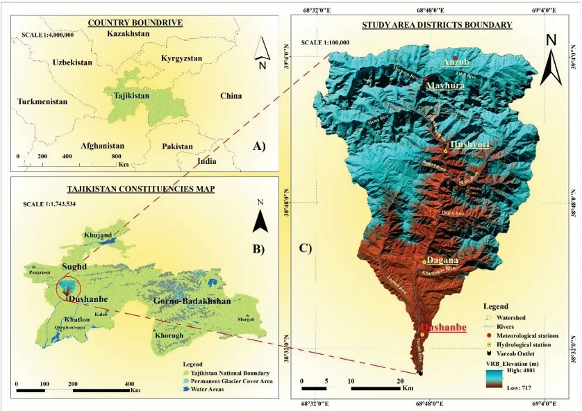
Fig. 1 A) Study area location; B) Physical map of Tajikistan; C) Varzob River basin.

According to calculations made based on remote sensing data (digital elevation map DEM), the area of the river basin. Varzob is 1723.48 km². The range of heights varies from 700m to 4800m above sea level. The Varzob River basin spans an area of 1723.48 km², with a glaciation level of 2.01%. The basin records an average annual water flow rate of 53.5 m³/s at the Putovsky Bridge. Additionally, the ice area within this basin has shrunk by 23.0%. The climate in Varzob river basin is characterized by significant precipitation during the winter period. The climate features include an average annual precipitation ranging from 500mm to 2000mm, with temperatures varying from -4°C to 18°C. Water discharge patterns peak seasonally, often in spring due to snowmelt or during rainy seasons. Its flow speed averages between 1.5 and 2.6 m³/s, and the primary water source is seasonal snow, with glaciers from high altitude areas contributing slightly (Gulayozov, 2022). The main contributing area lies in the upper Ziddi River, home to three glaciers, one stretching up to 4 km. Additionally, up to 10 smaller glaciers, each 1.5-2 km long, are found in the Mayhura River basin. Based on the calculation of glaciation from Landsat satellite images in 2001, it was determined that the total glacier area in the Varzob River basin is 26.97 km² (Gulayozov, 2022). Although glaciers are present in the upper basin, their impact on the river's flow is small due to the limited basin size. The river's flow significantly increases during the spring, peaking at 115 m³/s in June, while in winter, it drops to 15 m³/s (Gulayozov & Fazylov, 2022a). This pattern highlights snowmelt as the main river water supply contributor. The steep slopes and terrain across the basin make agricultural activities difficult. Settlements are limited to small areas near rivers and streams. Moving southward, the basin's elevation decreases, with the steep mountains transitioning into plateaus and then lowlands, which gradually become covered with loess soil.

The ASTER GDEM was utilized to create eight 500-meterwide elevation bands (Figure 2) for the river basin study area, excluding area A. These bands helped determine the average elevation for the targeted zone. The catchment area distribution across each altitudinal zone is displayed by the hypsometric curve in Figure 3, and the individual characteristics of the given zone are listed in Table 1. ArcGIS subdivided the watershed into eight separate elevation zones to model snow and glacier melt runoff with SRM. These zones range from 717 to $4500m$ in the catchment's DEM. Each zone has specific variables for calculating snowmelt runoff, as they vary with elevation. The Varzob River basin's eight 500-meter elevation bands allowed the calculation of mean elevation, which helped determine degree-day factors and coefficients for SRM modelling. Data on temperature and rainfall collected from three hydro-meteorological stations are converted to spatial data utilizing the Thiessen polygon method for weighted rainfall calculations in SRM.

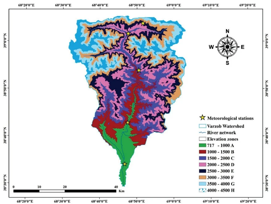
Fig. 2 DEM of the Varzob River basin showing the eight altitudinal zones used in this investigation.

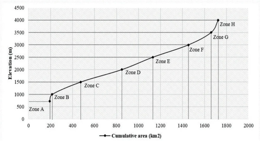
Fig. 3 Varzob River basin hypsometric curve showing the area in 8 elevation zones.

Table 1. DEM of Varzob River basin elevation zones

Zone	Elevation range (m)	Area (%)	Area ($k{m}^2$)	Cumulative area ($k{m}^2$)
A	717 - 1000	11.12	191.59	191.59
B	1000 – 1500	1.34	23.18	214.76
C	1500 – 2000	15.12	260.60	475.36
D	2000 – 2500	21.61	372.41	847.78
E	2500 – 3000	16.34	281.66	1129.44
F	3000 – 3500	18.82	324.28	1453.72
G	3500 – 4000	11.92	205.48	1659.20
H	4000 – 4500	3.73	64.28	1723.48
Total	717 – 4500	100	1723.48

2.2. Data sources

This study's climate and hydrological data include details on the mean/average annual temperature, annual precipitation, and annual runoff for the Varzob River basin. The climate data were sourced from five stations as shown in Table 2, provided by the Agency of Hydrometeorology under the Committee for Environmental Protection of the Republic of Tajikistan Hydrological data from this study were collected from Tajikistan's Ministry of Energy and Water Resources. To ensure the accuracy of the climate data, it was cross-verified with two external sources downloaded from www.pogodaiklimat.ru and www.snobear.colorado.edu, which supply hydro-climatic information for Central Asia. Some data gaps were found in the monthly temperature records: nine months were missing for the Anzob station, one month at the Hushyori station, and twelve months at the Mathura station. Regarding precipitation, the Anzob station had a nine-month gap, the Hushyori station had a two-month gap, and the Dushanbe station had a seven-month gap. The performance of classification algorithms depends heavily on data quality, and missing values can significantly reduce model accuracy. To address this, we used the K-Nearest Neighbor (KNN) imputation method to estimate missing data based on similar observations. Then, we evaluated the impact of imputation using the Naive Bayes classifier. Results showed that KNN imputation maintains classification accuracy close to that of complete datasets, demonstrating its effectiveness in handling missing data (Pujianto et al., 2019, Pan et al., 2010, García-Laencina et al., 2009). Furthermore, the accuracy and precision of the upstream runoff data were verified utilizing data from OSHC "Barqi Tojik" (http://www.barqitojik.tj/), which has observational points for measuring river runoff in the Varzob River basin.

Table 2. Location of climate stations under study, including their coordinates, along with monthly averages of air temperature (T), precipitation (P), and total water discharge (F) for each season

WMONo	Climate Station	Lat.(0N)	Lon.(0E)	Elev.(m)	T (°C)						P (mm)
					(Win.	Spr.	Sum.	Aut.)	Avg.	(Win.	Spr.	Sum.	Aut.)
38836	Dushanbe	38.35	68.44	800	4.02	15.26	26.18	15.02	15.1	81.9	101.8	8.4	30.6
38833	Hushyori	38.53	68.50	1361	0.47	10.95	22.32	12.33	11.5	143.2	170.5	25.8	70.8
38717	Mayhura	68.47	39.01	1922	-6.29	5.23	17.60	7.50	6.01	146.7	138.2	2.18	57.8
38719	Anzob	39.50	68.52	3373	-11.77	-2.96	8.32	-0.44	-1.7	52.3	55.4	19.1	25.4
WMONo	Discharge Station	Lat.(0N)	Lon.(0E)	Elev.(m)					Q($m^3/s$)
							(Win.	Spr.	Sum.	Aut.)	Avg.
17150	Dagana	38.59	68.77	1295			(14.10	73.65	89.21	19.32)	49.28

2.3. Snowmelt Runoff Model (SRM)

The WMO (World Meteorological Organization) has assessed SRM for runoff simulation and successfully replicated conditions for real-time runoff predictions (Organization, 1992, WMO, 1986). Equation 1 describes how the projected recession or decline flow is combined with water from rainfall and snowmelt to calculate the daily outflow from the basin:

where $Q=$ Average daily discharge [m${}^3$/3], $C=$ Runoff coefficient (runoff/ precipitation) expresses losses, with $c_S$ Snow melting and $c_R$ to rain, $a,=$ Degree-day factor [cm${}^0$C${}^{-1}$d${}^{-1}$]1${}^0$ day snowmelt depth, $\Delta T=$ Lapse rate adjustment while extrapolating station temperature to average basin or zone elevation [°Cd], $S=$ Snow coverage ratio, $P=$ Runoff-causing precipitation [cm]. Equation 1 assumes an 18-h lag between the daily temperature and discharge cycles.

The simulation for the Varzob River basin employed WinSRM version 1.12, a program designed to simulate snow and glacier melt runoff. Degree-Day Temperature Index has been applied to predict runoff from snow and glacier melt. Flowchart of the applied approach is provided in Figure 4.

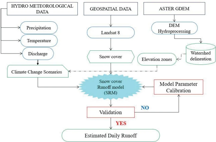
Fig. 4 Flowchart of the snow melt runoff model (SRM).

The meteorological network in the Hissar Ridge is subpar, offering only average data on temperature, precipitation, and water discharge. Temperature indices are the most accurate way to measure heat transfer during snowmelt and are widely used to determine melt rates. The complex energy balance causing snowmelt is evaluated using daily degree-days. A degree-day is defined as the total heat accumulated over a 24-hour period when the air temperature differs by 1 °C from a reference temperature. The most common Equation linking daily snowmelt to the temperature index is:

where $M=$ Water melted in cm/sec, $D_f=$ Degree-day factor ($c{m}^{0}Cda{y}^{-1}$), $Ti=$ Index air temperature(${}^{\circ }$C), and $T_b=$ Base temperature (usually $0^{\circ }$C)

2.4. SRM Parameters

In SRM, various parameters need to be defined for calibration and validation. The calibration and validation periods were from January 2015 to December 2015, January 2016 to December 2016, January 2017 to December 2017, and January 2018 to December 2018. After each run, the SRM automatically computes or counts and displays these as accuracy metrics. Table 3 presents the calibrated parameters and their corresponding values applied in basin-wide simulations. Daily runoff measurements from the Dagan hydrologic station were used to plot the discharge of a specific day $(Q_n)$ against the discharge of the subsequent day $(Q_{n+1})$ on a logarithmic scale. The recession coefficients $(X_c$ and $Y_c)$ are subsequently calculated from this $Q_n$ versus $Q_{n+1}$ plot. Therefore, the runoff coefficients presented in the following table vary by zone and month, reflecting the spatial and temporal variability of runoff across the study area. These coefficients were derived from a combination of rainfall and snowmelt contributions, which are considered together in the calculation process. Specifically, the coefficients account for both the amount and type of precipitation (rain or snow), as well as the timing and intensity of these events throughout the year.

Table 3. Range of parameter values used in the calibration of the SRM model

Parameters	Range		Description
	Min	Max
Temperature lapse rate °C/100m	0.65	0.65	Constant for all the zones
Degree-day factor $cm°C^{-1}{d}^{-1}$	0.65	0.65	Constant for all the zones
Critical temperature; TCRIT (°C)	2	2	Constant for all the zones
Time lag(hr)	18	18	Constant for all the zones
Runoff coefficient for snow, $C_S$	0.250	0.700	Varies month wise and zone wise
Runoff coefficient for rain, $C_R$	0.500	0.600	Varies zone wise
Rainfall contributing area, RCA	0	0	Constant for all the zones
$X_{coeff}$	1.0	1.02	Varies zones wise
$Y_{coeff}$	0.001	0.880	Varies zones wise

Treatment of glacierized zones, which is 2 % of our basin area, is an important step for successful basin modelling. The uppermost elevation belt (4 000–4 500 m) is glacierized but remains snow-covered until late July. Accordingly, the baseline model applies the snow degree-day factor ($DD{F}_{snow}=0.65cm{}^{\circ }{C}^{-1}{d}^{-1}$) throughout the year and does not activate the explicit glacier-melt routine. A sensitivity run that applies $DD{F}_{ice}=0.90cm{}^{\circ }{C}^{-1}{d}^{-1}$ and $K_{ice}=0.25$ once bare ice is exposed (August–December) changes peak discharge and annual runoff by less than 2 %, supporting the parsimonious baseline configuration.

2.5. Snow-Cover Estimation

In this study, we used Landsat 8 data to analyze snow coverage, utilizing a product that updates every 16 days in order to not miss any temporal data. Mapping snow cover was labor-intensive, requiring daily satellite images to be processed for snow extraction, provided the area was cloud-free. The large file sizes and numerous images posed challenges. From October 2015 to September 2018, we processed Landsat 8 images from Earth Explorer (https://earthexplorer.usgs.gov) on 13 November 2023. Each Landsat 8 image was in Geographic Tagged Image File Format (GeoTIFF) and WGS 1984 UTM Zone 42N projection for our study area Varzob Catchment. If cloud cover exceeded 10-20% on a given day, the image was discarded and snow coverage was estimated by interpolating between the nearest cloud-free images. Snow pixels were converted into square kilometers, and each 16-day interval was divided by the basin area and interpolated to estimate daily snow cover.

2.6. Model calibration and validation

It is necessary to calibrate and validate before implementing the provided model in real-world situations. This process ensures that the model accurately reflects observed values. The SRM model includes numerous parameters due to regional variations, which were determined through a calibration process since their direct obtaining from existing data is possible. In this study, calibration was done manually by adjusting input parameters. After calibration, thorough validation is necessary to test the model's performance under different conditions. The parameters set during calibration were used during validation, and the model's predictions were compared to the observed data. Calibration was based on data from the 2015 hydrological year, while data from 2016 till 2018 were used for validation.

2.7. Model Evaluation

The SRM computer program evaluates model accuracy by graphically comparing hydrograph estimation with observed runoff. Alongside these plots, SRM employs two performance indices: the percent volume difference $(D_v)$ and the coefficient of determination $(R^2)$ (Kushwaha et al., 2021, Martinec et al., 2008b, Shukla et al., 2021, Tahir et al., 2011, Vishwakarma et al., 2022). $R^2$ and $D_v$ , as defined below, are two criteria calculated by the model automatically (Martinec et al., 2008a).

Here, $R^2$ is a measure of model efficiency $[-]$, $Q_i$ is the observed daily Discharge $[m^3/s]$, $Q_j$ represents the daily discharge simulation $[m^3/s]$, $\bar{Q}$ represents the average daily Discharge for the season or year under simulation $[m^3/s]$, $n$ is the number of daily discharge values $[-]$, $D_v$ is the percentage difference between the total measured and simulated runoff $[\%]$, $V_R$ is the measured runoff volume $[m^3]$ and $V_{R^{\prime }}$ is the simulated runoff R volume $[m^3]$.

2.8 Climate Change Impact Detection

In high-altitude catchments, fluctuations in river flow reflect both the timing and distribution of precipitation and the temperature-driven melt of snow and ice. Because snowmelt supplies the bulk of runoff in the Varzob basin, this system is especially sensitive to climatic shifts: studies suggest that a 1–3 °C warming in the western Himalaya could increase glacier-melt runoff by 16–50 % (Singh et al., 1997). To explore how such changes might alter Varzob discharge, we employed the Snowmelt Runoff Model within the WinSRM framework. Rather than using standard global emissions pathways, we designed two bespoke scenarios for our simulations:

Scenario A: uniform 10 mm increase in precipitation

Scenario B: 2.5 °C rise in temperature

These tailored experiments will help quantify how precipitation and melt dynamics at high elevations could reshape runoff under future climate conditions.

2.9. Mann-Kendall Test

The M-K test is commonly used to identify trends in environmental, climate, or hydrological data (Patle et al., 2015). The main advantage of the M-K test is that the provided sample does not need to follow a particular statistical distribution. The M-K test's alternative hypothesis (H1) assumes an increase/upward or decrease/downward in the monotonic trend, whereas the original hypothesis (H0) states that there is no trend or serial correlation in the examined sample.

The M-K test statistic S is calculated as follows:

If $n$ is less than 10, we compare the absolute value of $S$ with the theoretical distribution of $S$ that M-K derived. A positive value of $S$ means that there is an upward trend, while a negative value indicates a downward trend. However, when $n$ equals 10, the $S$ statistic has a normal distribution and a mean of 0.

2.10. Wavelet analysis

The Morlet wavelet is defined as:

where $w_0$ is dimensionless frequency and $n$ is dimensionless time. The wavelet is stretched by varying its scale ($s$) so that $\eta =t/s$ and it is normalized to unit energy (Pan et al., 2020). Utilizing the Morlet wavelet analysis (with ${\omega }_0=6$) featuring a time-frequency multi-resolution function offers a favorable trade-off between time and frequency localization. The primary goal of the continuous wavelet transform (CWT) is to identify the primary oscillations of signals in the time-frequency domain. Central to wavelet analysis is the wavelet function, which belongs to a group of functions characterized by oscillations and rapid decay to zero. The CWT of time series $(x_n,n=1,\dots ,N)$ , sharing a uniform time step is defined as the convolution with a shifted and scaled factor of $x_n$ and normalized wavelet (Pan et al., 2020).

The CWT is shown below as:

The basic principle of wavelet analysis can be known from Equation (8). The discrete continuous wavelet transform coefficient is computed at time index $n$ and scale $s$. Here, $\delta t$ is the sampling interval of the time series, $s$ is the dilation (scale) of the mother wavelet ${\psi }_0$, $N$ is the total number of data points, and $x_n^{\prime }$ is the signal amplitude at index $n^{\prime }$. The argument $(n^{\prime }-n)\frac{\delta t}{s}$ represents the nondimensional time shift, and the factor $\sqrt{(\delta t/s)}$ normalizes the transform's energy. The low-frequency or high-frequency information of the signal is obtained by increasing or decreasing the scaling scale $a$ and then analyzing the profile or details of the signal to achieve different local time characteristics and spatial characteristics of the signal analysis (Labat, 2010). In other words, CWT applies wavelet as a band pass filter to time series. CWT can clearly reveal the various oscillation period hidden in the time series, fully reflect the variation trend of the system in different time scales (Pan et al., 2020).

3. Results and Discussion

3.1. Model Performance

The Snowmelt Runoff Model was applied to simulate snowmelt-driven runoff within the catchment area. At the start of the melting period, water losses are minimal, mainly consisting of evaporation from snow cover. However, evapotranspiration and vegetation interception cause water losses to significantly increase as snow continues to melt and vegetation growth starts. Using discharge data from the 2015 hydrological year, the model was first run with default parameters and no modifications, and the results were recorded. Model performance was evaluated daily by comparing simulated and observed streamflow through graphical analysis. Additionally, model accuracy was quantified using volume difference ( $D_v$ ) values between simulated and observed Discharge. Figure 5 illustrates the comparison of simulated and observed monthly discharge values prior to calibration. Overall, the model overestimated Discharge, particularly during peak snowmelt months. The coefficient of determination $R^2$ value obtained for the pre-calibration run was 0.6924, with the highest discharge levels recorded in April.

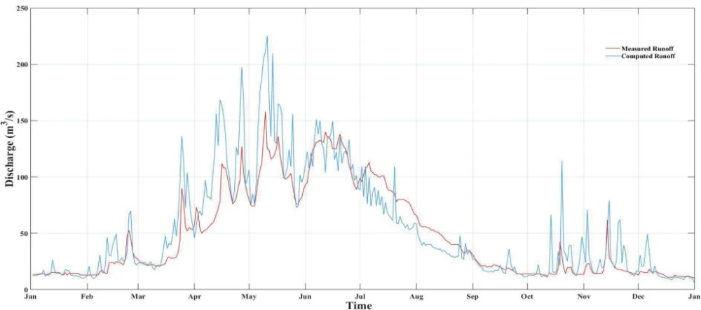
The SRM model for 2015 was manually calibrated by repeatedly running it to find the watershed's ideal degree-day parameter value, which was found to be $0.65m{d}^{-1}{\mathrm{o}\mathrm{C}}^{-1}$. Through multiple iterations, optimal values were also established for critical temperature, lag time, and recession coefficient parameters. Table 4 presents the SRM snowmelt runoff calibration and validation results. It can be seen from the table, that the ${ℝ}^2$ values during the simulated period from January 2015 to December 2018 are 0.9357, 0.8558, 0.9588, and 0.9492. Observed runoff during this time ranges from 1518.394 to 1237.546 million cubic meters $m^3({10}^6{m}^3)$, with an average flow of 48.148 to 39.242 cubic meters per second $(m^3/s)$. Calculated runoff varies between 1502.953 and 1240.97 million cubic meters $m^3({10}^6{m}^3)$, with average flows of 47.657 to 39.351 cubic meters per second $(m^3/s)$. The volume difference from 2015 to 2018 ranges from $1.0169\%$ to $-0.2767\%$.

Table 4. Results of model simulation for the period 2015-2018 for the Varzob River basin

Period	Runoff Volume$({10}^6{m}^3)$		Average Runoff$Q(m^3/s)$		VolumeDifference, $D_v($	Coefficient ofDetermination, $R^2$	Nash-Sutcliffe coefficient (NSE)
	Measured	Computed	Measured	Computed
2015	1518.394	1502.953	48.148	47.658	1.0169	0.9357	0.8745
2016	1495.74	1452.398	47.3	45.929	2.8977	0.8558	0.8926
2017	1477.829	1471.156	46.862	46.65	0.4516	0.9588	0.9012
2018	1237.546	1240.97	39.242	39.351	0.2767	0.9492	0.8964

Once calibrated, the model could be directly applied to subsequent years by updating only the input data without altering the calibrated parameters. The model was validated annually for the hydrological years from 2015 to 2018, using the parameters established during calibration. Figure 6a compares the simulated and observed discharge values for 2015, showing a close alignment between them. The highest discharge value occurred in May( $158.0m^3/s$ ). In 2015, the model performance indicators reflected good overall performance despite slightly overestimating Discharge, which remained within acceptable limits. The validation results confirm a strong match between simulated and observed values, with statistical parameters falling within a satisfactory range.

The model was also applied to 2016, with the validation run showing the highest Discharge in July (209.0 $m^3/s$). Figure 6b compares the simulated and observed discharge values, demonstrating strong agreement with a $D_v$ of $2.8977\%$ and $R^2$ of 0.8558 and NSE with 0.8926. Similarly, the SRM model was executed for 2017, with the results shown in Figure 6c. The result demonstrates good model performance, with the highest Discharge occurring in April (137.0$m^3/s$). The modeled and observed values for 2017 matched well, with $0.4516\%$ and 0.9588 and 0.9012 of NSE. For 2018, the comparison between simulated and observed values Figure 6d indicated excellent agreement, with a $D_v$ of $0.2767\%$ and 0.9492 and 0.8964 were recorded as NSE. The highest discharge in 2018 occurred in May (105.00$m^3/s$), differing from previous years due to significant flooding.

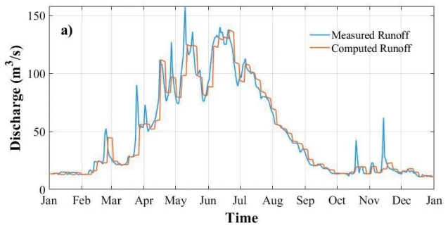
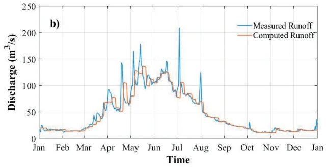
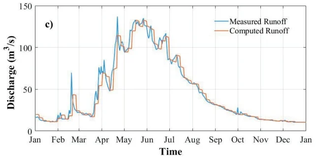
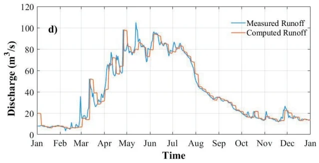
The annual statistical error results from 2015 to 2018, including calibration and validation periods, show that overall, the model performed exceptionally well. Nevertheless, the model occasionally exhibited periods of streamflow overestimation and underestimation. When compared to earlier research done in other parts of the world, the agreement between the modeled and observed values was noticeably high (Butt & Bilal, 2011, Prasad & Roy, 2005). The average $R^2$ and $D_v$ values for the entire simulation period were 0.923 and $1.022\%$ and 0.8911 respectively, closely aligning with the results obtained during the calibration and validation phases. These statistical measures attest to the SRM model's outstanding accuracy in this investigation, indicating that it might successfully support water resource management and planning initiatives by simulating runoff in other Hissar Ridge basins.

3.2. Climate Change Impact on Streamflow

A simulation period spanning January to December 2015 was chosen to evaluate the impacts of climate change under two different scenarios. Figure 7 depicts the discharge variations using change ratio under these scenarios throughout the 2015 hydrological year, while Table 5 summarizes monthly discharge simulations. In Scenario A, the results indicate that summer streamflow is likely to increase with snow cover expansion. Assuming a constant mean temperature, a 10 mm rise in precipitation would lead to an approximate 9.57% (280.9 m³/s) increase in average discharge during the summer months (June to August), compared to the current average of 256.4 m³/s (Xie et al., 2018). The highest peak discharge for the simulated year occurred in June, reaching 119.2 m³/s; with the 10 mm precipitation increase, the peak discharge rose to 125.0 m³/s. In Scenario B, as depicted in Table 5, a 2.5 °C rise in temperature resulted in a 5.47% (270.5 m³/s) increase in average summer discharge. The peak discharge for this scenario also occurred in June at 119.2 m³/s. However, with a temperature rise of 2.5 °C, the peak discharge was slightly reduced to 125.1 m³/s in June.

Table 5. SRM simulation under climate change scenarios with modified precipitation and temperature inputs

Climate Change Run	Simulated Discharge of 2015($m^3/s$)	Simulated Discharge ($m^3/s$)
		With 10mm Increase in Precipitation	With Temperature +2.5°C
January	13.5	14.1	13.7
February	23.1	25.4	22.3
March	33.9	38.5	32.9
April	77.5	85.2	76.8
May	102.1	115.1	106.7
June	119.2	125.0	125.1
July	90.6	95.3	99.4
August	46.7	50.2	56.3
September	19.8	21.6	27.3
October	16.7	17.5	21.0
November	20.5	21.1	21.7
December	13.3	14.7	14.4

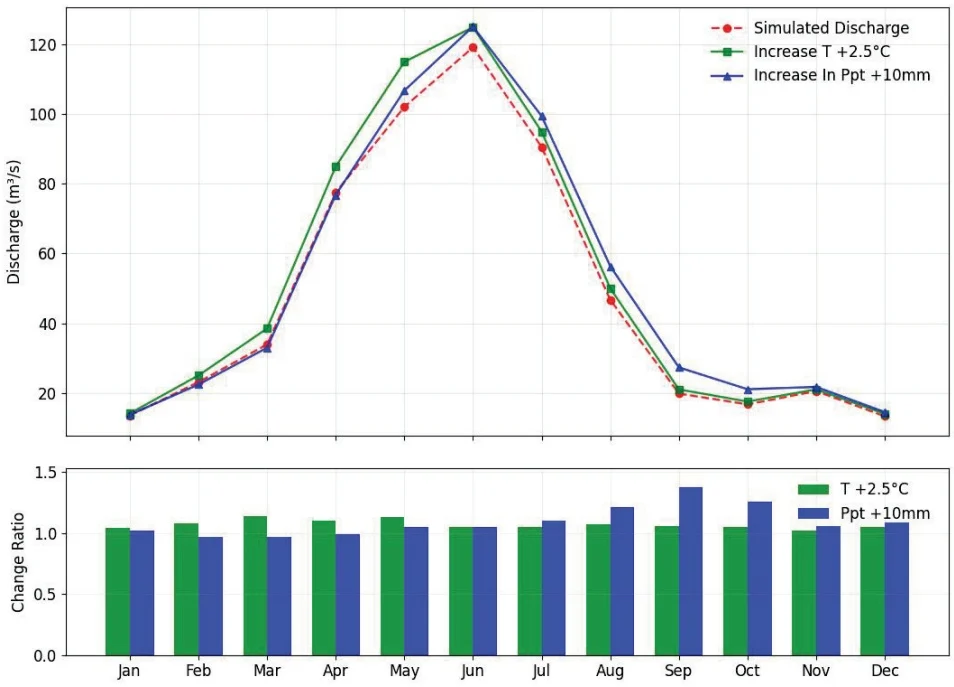
Fig. 7 (a) Monthly discharge hydrographs of climate change scenarios against simulated, (b) Scenarios to simulated discharge ratios for the year 2015

In this study, 2015 was the reference year for the climate scenarios discussed. The results indicate that spring streamflow is anticipated to decline with an increase in mean temperature or precipitation, while summer streamflow is expected to rise with increased precipitation or temperature.

3.3. Monthly, Seasonal and Annual Trends for Temperature and Precipitation

The Z statistics for monthly temperature and precipitation data, obtained using the Mann–Kendall test, are shown in Table 6 and Table 7 respectively. A positive Z value indicates an upward trend, while a negative Z value indicates a downward trend. The test determines the minor significance level $\alpha$ at which the null hypothesis of no trend can be rejected. For the four tested significance levels, the following symbols are used: $\otimes$ for a trend at $a=0.001$ , $\oplus$ for $\alpha =0.01$, $\circ$ for $\alpha =0.05$ and $+$ for $\alpha =0.1$. If a cell is blank, the significance level is greater than 0.1, indicating that the trend is not statistically significant at those levels.

Table 6. Z Mann–Kendall test statistics for monthly temperatures every station

Climate Station	Statistics on Mann-Kendall Trends
	Test Z	P Value	Significance Level	Sen's Slope
Dushanbe	2.9186	0.0035	⊕	0.4706
Hushyori	3.0251	0.0025	⊕	0.5432
Mayhura	2.2689	0.0233	○	0.4286
Anzob	3.2870	0.0010	⊗	0.5253

Table 7. Z statistic of Mann–Kendall test for monthly precipitation for every station

Climate Station	Statistics on Mann-Kendall Trends
	Test Z	P Value	Significance Level	Sen's Slope
Dushanbe	-0.1867	0.8519		-0.0577
Hushyori	-1.7333	0.0830	+	-0.3492
Mayhura	-0.6144	0.5389		-0.1464
Anzob	1.6810	0.0928	+	0.3069

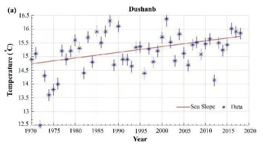
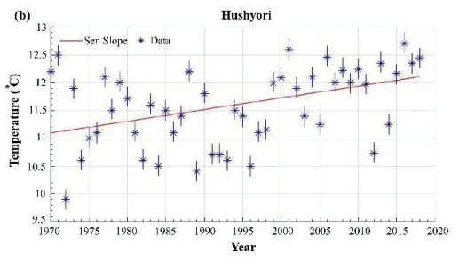
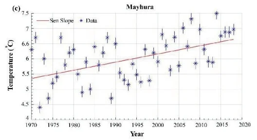
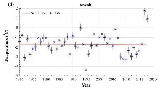
Using the nonparametric modified Mann-Kendall test, trends and magnitude changes in annual air temperature, precipitation, and water discharge were computed for data from multiple stations across the Varzob River basin. The temperature data for Dushanbe station (Figure 8a) from 1970 to 2018 alternates between around ${12}^{\circ }C$ and ${16}^{\circ }C$. It can be noted that 1972 and 2001 have the lowest and highest annual temperatures at ${12.50}^{\circ }C$ and ${16.37}^{\circ }C$. An upward trend can be observed in both the trend line and the Mann-Kendall (M-K) test, with a 99% confidence interval confirming the upward trend (Table 6). At the Maykhura station (Figure 8c), the annual temperature increases, with the highest temperatures coming at the end of the period. The MK test confirmed the trend in the data with a 95% confidence interval as shown in Table 6. Anzob station data (Figure 8d) showed varying temperatures from -4.5 °C to 1.76 °C. A sharp fall in temperature can be spotted in 1995 and 2008. Interestingly, both drops come after the high-temperature years 1994 and 2006, respectively. The MK test results show sufficient evidence to reject the null hypothesis with a 99.9% confidence interval (Table 6). Thus, there is an upward trend. The temperature in the Hushyori station (Figure 8b) can alternate between 9.9°C and 12.70°C. The trend line in the graph can be seen to have an upward trend distinctly. The MK test confirmed the presence of a trend in the data at 99% (Table 6).

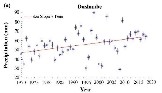
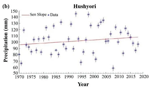
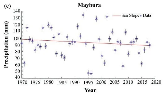
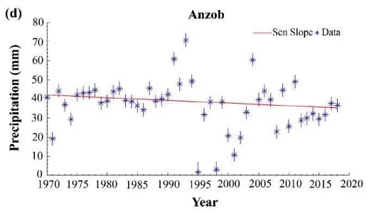
The monthly precipitation data at the Dushanbe station from 1970 to 2018 indicated no significant trend (Figure 9a). Even though the Sen Slope looks like having an upward trend, no statistically significant trend was identified (Table 7). Similarly, data at the Mayhura station is highly volatile and was not confirmed to have a significant trend (Figure 9c). However, at Hushyori station a statistically significant upward trend (Figure 9b) could be detected at $90\%$ confidence level (Table 7). Similarly, data from the Anzob station indicated the presence of a downward trend (Figure 9d) at $90\%$ confidence level. The precipitation data shows high volatility at all the stations.

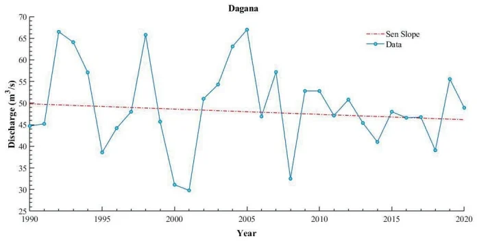
Fig. 10 Trend statistics and Sen Slope of the annual water discharge over the period 1990-2018 at the Dagana station.

MK test of the water discharge's annuals records at the Dagana station from 1990-2016 indicated the absence of a trend (Figure 10).

3.4. Continuous Wavelet Transform Seasonal patterns

A continuous wavelet transform (CWT) was used to identify the oscillations in the data. The Morlet wavelet was chosen among other wavelets as it has often been used to analyze complex environmental signals. The CWT indicates a strong one-year periodicity in the monthly temperature data at the Dushanbe station over the entire observation period, as seen in (Figure 11b). At the Mayhura station, a one-year cycle for temperature can be identified over most of the observation period from 1970-2018 (Figure 11a). The CWT of monthly temperature data at the Anzob hydro stations displays a strong one-year cycle over the entire observation period (Figure 11d). It can also be noted that the one-year oscillation is less intense during the first half of observation and gets stronger over the second part from 2008-2016. The CWT showed a prominent one-year cycle for monthly air temperature for the entire observation period at the Hushyori station (Figure 11c).

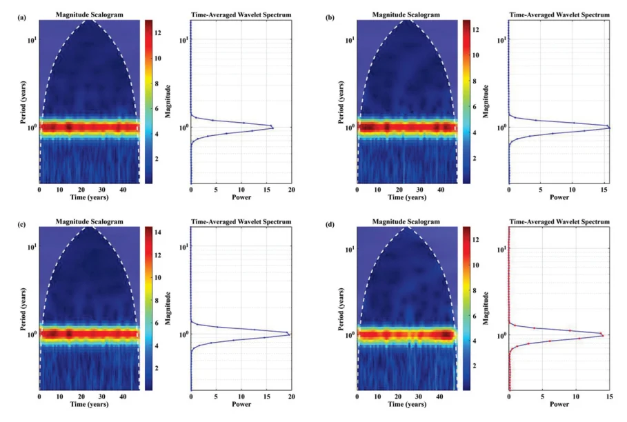
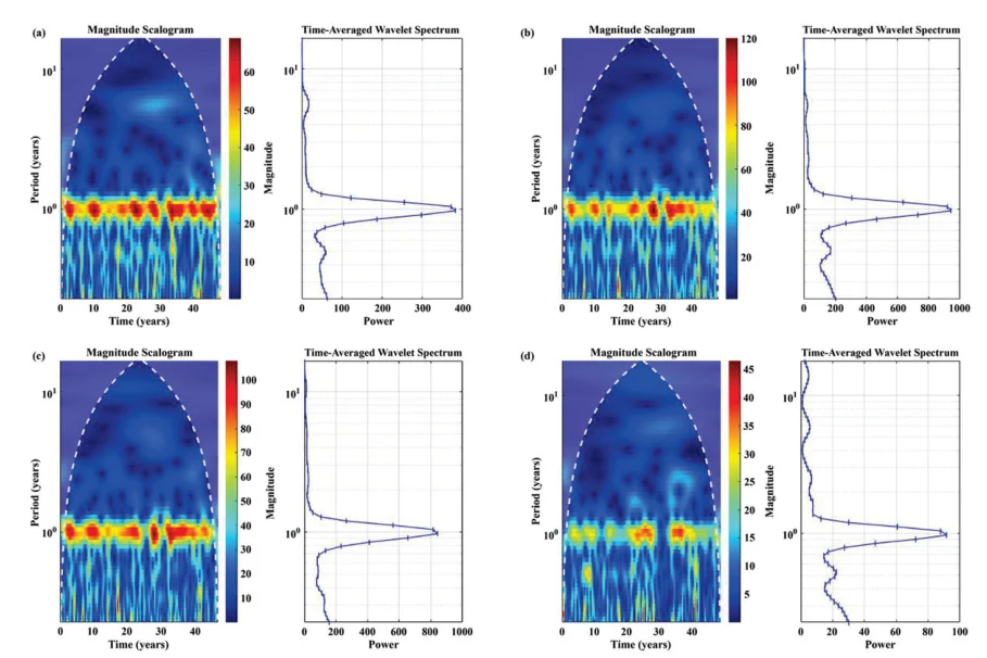
Mayhura station's precipitation data showed a strong one-year periodicity over the entire observation period, with a gap of 1 year after 2000 (Figure 12a). At the Dushanbe station, precipitation data displayed a one-year periodicity with gaps around 1995, 2000, and 2012. Additionally, the periodicity was less prominent during the last quarter of the observation period from 2010 to 2016 (Figure 12b). Precipitation data at the Anzob station showed a one-year cycle from 1992 to 1998 and 2005 to 2008. A less intense one-year cycle was also present from 2009 to 2015 (Figure 12d). The CWT of precipitation data at Hushyori showed a one-year periodicity through most of the observation period (Figure 12c). The cycle is less prominent around 1995, 2001, and 2012. It is also worth noting that the power of the period was less prominent over the last period from 2010 to 2016.

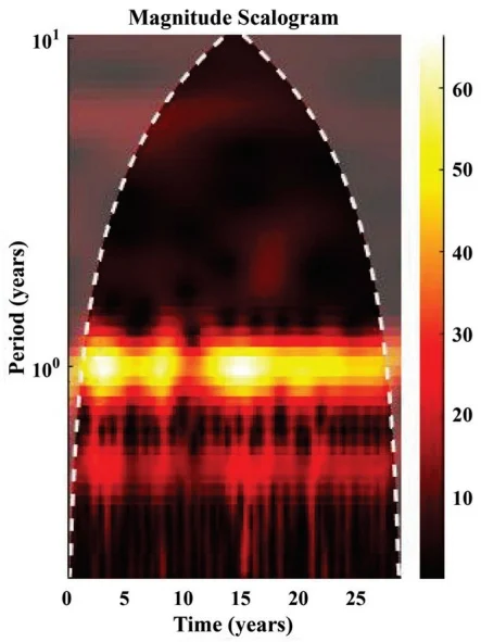
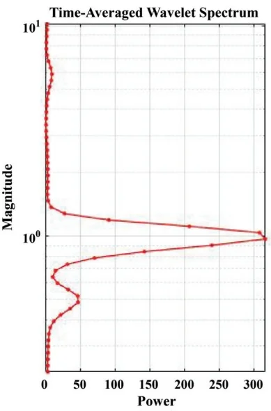
The continuous wavelet transforms for monthly water discharge over 27 years from 1990 to 2018, showing a periodicity of 1 year (Figure 13). It can be distinctly identified on the time-averaged wavelet power spectrum. However, it is less prominent during the 1999-2002 years. Additionally, a minor 6-month cycle was identified over the observation period. Additional plots are presented in the Appendix I. Figures 16-17 in Appendix I show the dominant periodicities of temperature data and wavelet spectrum with significance testing at 95% level. Wavelet analysis of temperature records from four stations (Anzob, Hushyori, Dushanbe, and Mayhura) between 1970 and 2018 revealed site-specific dominant periodicities that reflect varying climatic influences. Both Anzob and Dushanbe exhibited pronounced decadal-scale signals, with dominant cycles of 14.8 and 18.5 years respectively, indicating a strong influence of long-term climate oscillations such as the PDO (Pacific decadal oscillation) and NAO (North Atlantic oscillation), supported by moderate persistence in their temperature time series. In contrast, Hushyori and Mayhura both exhibited dominant periodicities of 8.6 years, aligning with the 7–11 year band typically associated with solar cycle variability. However, their relatively low persistence suggests that these solar-related influences, though present, are superimposed by more irregular variability. No significant ENSO (El Niño–Southern Oscillation) -related (2–4 year) signals were detected at any station, nor were decadal oscillations apparent at Hushyori and Mayhura. Collectively, these results highlight that while temperature variability at Anzob and Dushanbe is predominantly governed by decadal climate modes, solar cycles play a more significant role at Hushyori and Mayhura. Understanding these differences is critical for interpreting historical climate variability and developing tailored adaptation and resource management strategies across the region.

In Appendix I the additional wavelet plots for precipitation data are shown in Figures 18-19. Wavelet analysis of precipitation records from four stations (Anzob, Hushyori, Dushanbe, and Mayhura) in the region from 1970 to 2018 revealed distinct dominant periodicities, reflecting varying climate influences across the sites. Anzob exhibited a dominant 14.8-year decadal-scale cycle, likely associated with large-scale oscillations such as the PDO or NAO, while Mayhura showed a primary periodicity of 11.1 years, suggesting influences from both the solar cycle and decadal climate variability. In contrast, Dushanbe's dominant 6.2-year cycle falls between the ENSO and solar cycle ranges, indicating the potential interplay of intermediate-term regional and global climate drivers. Hushyori displayed a principal cycle of 4.9 years, just outside the ENSO band, pointing to the importance of interannual variability but with limited influence from longer-term oscillations. Across the stations, AR1 coefficients ranged from negative to weakly positive, indicating generally low persistence and suggesting that these periodicities are superimposed on substantial irregular variability. Collectively, these findings highlight the spatial diversity of climate influences on precipitation across the region, with some sites primarily affected by decadal or solar-related cycles, while others are governed by shorter-term or intermediate climate patterns. Understanding these site-specific periodicities is crucial for improving regional water resource management, forecasting, and adaptation strategies.

Water discharge supplementary plots can be found in Appendix I in Figures 20-21. Wavelet analysis of the water discharge data from the Dagana station for the period 1990–2020 identified a dominant periodicity of 6.2 years. This intermediate timescale does not align directly with the typical ENSO band (2–4 years) but lies just below the 7–11 year range often attributed to solar cycle influences. The presence of a 6.2-year dominant period suggests that water discharge at Dagana may be influenced by regional or global climate patterns that operate on multi-year scales, potentially through the interaction or overlap of ENSO and solar-related cycles, or by regional hydrological processes with similar periodicity. The AR1 coefficient of 0.234 indicates moderate persistence in the discharge series, reflecting the presence of sustained multi-year fluctuations rather than purely random variations. The absence of significant signals in the decadal or ENSO bands implies that while classic global drivers may contribute, the main variability in discharge is governed by processes operating on intermediate timescales. Recognizing this dominant 6.2-year cycle is important for understanding river regime variability and can inform water resource management, flood risk assessment, and planning in the Dagana catchment.

3.5. Snow Cover

Table 8 presents the Snow Cover Area (SCA) percentage obtained from Landsat 8 imagery captured on coinciding dates. The maximum value of 44.91% occurred on 22 January 2016, while the minimum value 0.23% was recorded in 5 September 2017. Figure 14 provides a detailed view of snow cover distribution across all zones within the Varzob River watershed, from 2015 through 2018. Figure 15 indicates that snow cover was lowest during August and September and highest during December, January, and February across all studied zones.

Table 8. Total Snow Cover Area (%) in the Varzob River Sub-basin Derived from Landsat 8 Imagery

Date of Images	Snow cover Area (%)Landsat 8
2 October 2015	11.96 (%)
22 January 2016	44.91 (%)
5 September 2017	0.23 (%)
24 September 2018	3.45 (%)

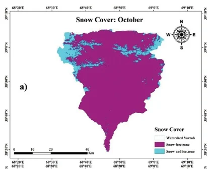
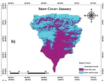
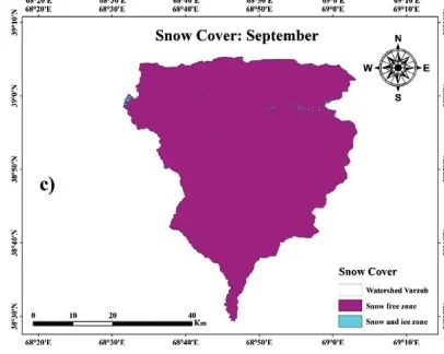
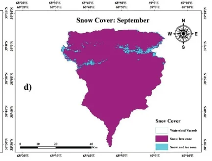
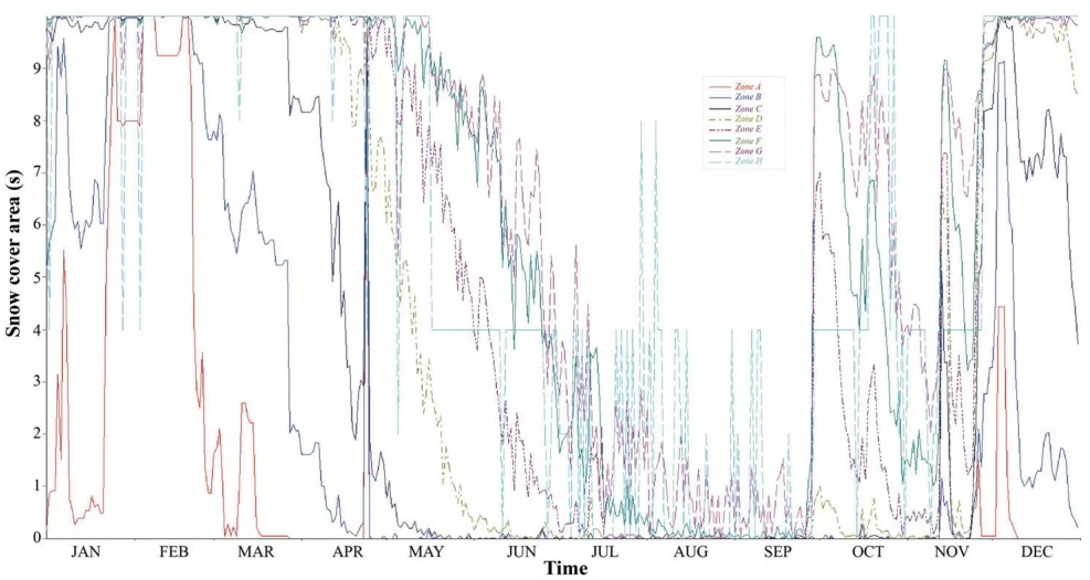
Fig. 15 Snow cover distribution in the Varzob River watershed during 2017.

3.6. Discussion

3.6.1 Climate Change Effects on Temperature, Precipitation, Glaciers, and Water Availability

The SRM exhibited robust predictive performance, achieving coefficient of determination ( $R^2$ ) values ranging from 0.8558 to 0.9588 during validation. Despite its overall accuracy, the model tended to overestimate discharge, particularly during peak melting seasons, reflecting the challenges of accurately capturing the complexities of hydrological responses to climate variability. This inconsistent precipitation pattern complicates water availability predictions, highlighting the uneven response of climate change scenarios to river hydrology regime. Further, the scenario modelling results indicate significant impacts on water availability. Under Scenario A (precipitation increase of 10 mm), average summer discharge increases by 9.57% compared to the baseline conditions, matching findings by Xie et al. (2018) who reported similar discharge increases ( $~$ 10-15%) in comparable basins under increased precipitation scenarios. Scenario B, with a 2.5°C temperature rise, showed negligible overall changes (5.45% increase) in summer discharge, although peak discharge reduced slightly from 119.2 m ${}^3$ /s to 125.0 m ${}^3$ /s, indicating an altered runoff regime potentially affecting peak water availability periods. The selected climate change scenario of a +2.5°C increase in temperature and +10 mm change in precipitation is based on regional projections aligned with IPCC AR6 scenarios and downscaled climate model outputs for Central Asia. Studies show that mean annual temperatures in high-mountain Asia are projected to rise between +2°C and +4°C by mid-century under SSP 2–4.5 and SSP 5–8.5 pathways (IPCC (2021). Regional assessments in the Pamir and Tien Shan ranges suggest comparable trends, with moderate increases in precipitation ranging from 5–15% by 2050 (Sorg et al. 2012; Hock et al., 2019). Our choice represents a mid-range, plausible climate trajectory to assess hydrological sensitivity in the study basin. The results also indicate significant warming trends within the Varzob River basin, with Mann–Kendall Z statistics ranging from 2.269 to 3.287 (P < 0.05), highlighting statistically significant warming at stations like Dushanbe, Hushyori, Mayhura, and Anzob. Sen's slope estimates quantify the magnitude of temperature increases, ranging between 0.429°C/decade (Mayhura) and 0.543°C/decade (Hushyori). These findings align quantitatively with regional studies, such as Bolch 2007; Gulahmadov et al. 2023) who found a significant increasing trend in temperature for the Varzob River basin and Northern Tien Shan region of Central Asia, during the periods 1950–2000, as well as 1960–2018 and 1991–2018.

We used the K-Nearest Neighbor (KNN) method to impute missing meteorological data, which estimates missing values based on similar observations. This method is widely used for its simplicity and effectiveness, maintaining classification accuracy close to that of complete datasets (Zhu et al. 2015; Troyanskaya et al. 2001; Müller et al. 2018; Li et al. 2013). However, KNN imputation can introduce biases, particularly under rare or extreme climatic conditions, potentially affecting model accuracy. While KNN is effective for moderate levels of missing data, its performance may degrade with higher missing rates, especially when temporal and spatial correlations are not well preserved (Choudhury et al. 2020; Feng et al. 2021; Zhang et al. 2020). Though we validated our imputed dataset with external sources, residual uncertainties may still influence the model's output, especially in data-scarce regions or extreme climate scenarios. Conversely, precipitation trends show limited statistical significance, with only minor upward (Sen's slope: 0.3069 and P < 0.1 at Anzob) or downward trends (Sen's slope: -0.3492 and P < 0.1 at Hushyori). This inconsistent precipitation pattern complicates water availability predictions, highlighting the uneven response of hydrological systems to climate change. Cloud cover remains a key limitation in snow cover estimation using Landsat 8, as it can obscure surface features and lead to temporal data gaps (Stillinger et al. 2019). Although Landsat offers superior spatial resolution (30 m), its 16-day revisit cycle increases the risk of missing critical snow events, especially in mountainous regions with frequent cloud cover. These gaps can cause underestimation or overestimation of snow-covered area (SCA), directly influencing SRM outputs (Foga et al. 2017). While gap-filling approaches or multi-source data integration may help, uncertainties remain particularly during rapid accumulation or melt periods. Consequently, we recognize that cloud-induced limitations in the Landsat record may contribute to residual uncertainty in modeled runoff estimates.

As shown by the calculations for the Varzob River basin, snow-melt supply has the largest share in the annual runoff, accounting for 60-70% of the annual runoff. Subsurface flow accounts for 20-25% of the annual runoff. The share of glacial supply in the total runoff is directly dependent on the degree of glaciation of the basin and the average height of the catchment area. Accelerated glacier thawing, driven by natural temperature trends combined with the greenhouse effect, further intensifies hydrological impacts. Rising temperatures increase meltwater production beneath glaciers; however, meltwater input fails to keep pace with meltwater loss, expediting glacier retreat. This enhanced degradation significantly reduces glacier coverage, compounded by direct melting. Yakarcha glacier and other glaciers in the Varzob River basin, along with those in Khanaki, Karataga, and Kafirnigan, are projected to disappear entirely due to their limited size and thickness. Consequently, river runoff will transition from predominantly snow-glacial sources to snow-rain and purely snow-driven regimes. From July to September, river flow will primarily depend on spring water and sporadic rainfall, significantly reshaping seasonal water availability patterns. While sufficient water supply may remain available for Dushanbe city, shortages are anticipated for irrigation systems and the operation of the Varzob cascade hydroelectric stations (Main Tajik Hydro-Meteorological Service, 2003). Two main factors identified for glacier area reductions include methodological accounting practices that incorporate snow-covered upper glacier zones at winter's end and increased air temperatures resulting from climate change.

Continuous wavelet transforms analyses quantitatively confirm prominent seasonal (1-year) periodicity in temperature and precipitation across stations, although weakened periodicity in recent years suggests growing instability in climate conditions. For instance, periodicity disruptions noted around 2010-2016 (Dushanbe, Hushyori) reflect increased variability and unpredictability in seasonal patterns. Analysis of daily discharge at Dagana station reveals an essentially flat (slightly negative), non-significant annual trend. Major flood-level events ( $\ge 60m^3{s}^{-1}$ ) occurred five times between 1989 and 2005 (1992, 1994, 1999, 2004, 2006), but only once after 2006, indicating no increase—and possibly a decline—in the frequency of extreme flows. Meanwhile, post-2010 flows remain clustered around the long-term mean, with moderate peaks generally confined to 40–55 m ${}^3$ s ${}^{-1}$, giving the record a “flattened” appearance and suggesting dampened variability rather than heightened susceptibility to extremes.

The study's findings highlight the intricate ways climate change affects the water systems in the Varzob River basin. Notably, there are clear upward trends in air temperature across multiple observation stations, whereas precipitation trends remain inconsistent. Scenario modeling underscores the significance of these variations, demonstrating that even minor climate variations (precipitation increases of 10 mm or temperature rises of ${2.5}^{\circ }$ C) can lead to substantial shifts in seasonal discharge patterns. This highlights the basin's sensitivity and emphasizes the necessity of adaptive water management strategies in response to climate change. These results have practical implications for resource management in the basin, where water availability directly impacts agriculture, hydropower, and urban supply. Strengthening snow and runoff monitoring systems, implementing early melt-season forecasts, and adopting flexible water allocation policies can support more resilient water governance. Moreover, integrating scenario-based planning within the existing water management framework can help decision-makers address future uncertainties. Such adaptive approaches will be particularly critical in other mountain catchments facing similar climate-induced hydrological variability.

3.6.2 Modeling Challenges and Implications for Water Management

The Snowmelt Runoff Model (SRM) demonstrated strong predictive accuracy, with coefficient of determination ( $R^2$ ) values consistently above 0.85 (ranging from 0.8558 to 0.9588 during validation). However, a consistent quantitative overestimation of discharge during peak melting seasons highlights modeling limitations under changing climatic conditions. Scenario simulations indicate even small climate shifts (precipitation ±10 mm, temperature +2.5°C) which significantly influence water availability, emphasizing the necessity for adaptive and proactive water management strategies. Quantitative assessments highlight urgent needs for improved hydrological forecasting, glacier and snow monitoring infrastructure, and capacity-building to handle increased runoff variability. Effective adaptation thus requires integrating climate and hydrological indicators into robust water resource planning frameworks to sustainably manage Varzob River basin’s water resources amidst increasing climatic uncertainties.

3.6.3 Model Limitations and Uncertainties

The SRM model has demonstrated effectiveness in simulating glacier- and snowmelt-driven runoff. However, its performance under extreme or non-linear climatic conditions (e.g., abrupt warming or altered precipitation regimes) remains limited. A key constraint is the assumption of constant degree-day factors (DDFs), despite their known variability across space, time, and snowpack conditions, which can lead to significant uncertainty in melt estimates, particularly during anomalous years. Remote sensing-derived snow cover inputs also introduce uncertainty due to cloud contamination, misclassification between snow and glacier ice, and coarse resolution, all of which may propagate errors in runoff simulations. Additionally, the model lacks explicit representation of key hydrological processes such as subsurface flow, glacial lakes, and permafrost dynamics, reducing its ability to capture short-term variability and complex glacier behavior. While calibration with the observed discharge data helps reduce these uncertainties, they remain important considerations especially in scenario-based analyses under changing climate conditions.

4. Conclusion

Studies on snow cover are crucial for hydrological and climatological research, especially in mountainous areas like the Varzob River basin. This study applied the Snowmelt Runoff Model (SRM) using daily temperature, snow cover, and precipitation data to simulate runoff in the Varzob catchment. The comparison of simulated and observed runoff values during the calibration and validation periods (2015-2018) demonstrated the SRM model's strong performance, with values of 0.9357, 0.8558, 0.9588, and 0.9492 for each respective year. Corresponding volume difference values for these years were 1.0169%, 2.8977%, 0.4516%, and 0.2767%. Additionally, the NSE also obtained the following values 0.8745, 0.8926, 0.9012, 0.8964 for each year respectively. The average value across all years was 0.925, and the average volume difference was 1.022%. These statistics indicate that the SRM model was highly effective in capturing the dynamics of snowmelt runoff.

The model results also revealed how future climate scenarios might impact the basin's hydrology. For example, a 10mm increase in precipitation could lead to a 9.57% rise in runoff, while a 2.5°C rise in temperature resulted in only a minimal increase in overall discharge (5.47%). Interestingly, the peak discharge in June increased from 119.2 m³/s to 125.0 m³/s with the temperature increase, and the same peak increased to 125.1 m³/s under the 10mm precipitation rise scenario. These findings indicate that changes in both precipitation and temperature can significantly influence runoff dynamics, with precipitation having a more pronounced impact on overall discharge volumes and peak flow, highlighting the basin's higher sensitivity to changes in moisture availability compared to temperature alone. The SRM model has proven effective in quantifying snowmelt runoff and simulating associated hydrological, climatic, and ecological processes, particularly in ungauged and mountainous areas. However, the model's tendency to overestimate discharge during the melting season points to the need for continued refinement, including better parameterization of factors like evapotranspiration and soil moisture dynamics. This study findings underscore the importance of ongoing research into snow cover and its relationship to regional hydrology under a changing climate. As snow cover expands or contracts, streamflow dynamics in spring and summer are directly affected, highlighting the need for adaptive strategies in water management. Improved forecasting and monitoring systems and an infrastructure capable of managing increased variability in water flow will be critical in ensuring sustainable water availability for both agricultural and domestic uses. Ultimately, the resilience of the Varzob River basin to climate change will depend on proactive, science-driven strategies that integrate hydrological modeling, climate forecasting, and adaptive management practices.

Author Contribution

All authors were involved in the intellectual elements of this paper. Conceptualization, Q.A., X.C., M.G. and T.L.; methodology, Q.A., X.C., M.G. and T.L.; formal analysis, Q.A., X.C., M.G., T.L. and F.M.; investigation, Q.A., X.C., M.G., T.L. and F.M.; resources, X.C. and T.L.; writing-original draft preparation, Q.A., X.C., M.G. and T.L.; writing-review and editing, F.M., F.A., D.Y., Z.K., H.L. and S.O.; visualization, Q.A.; supervision, X.C. and T.L.; All authors have read and agreed to the published version of the manuscript.

Acknowledgements

The first author is very thankful to the University of Chinese Academy of Sciences (UCAS) Scholarship program (http://english.iue.cas.cn/et/scs/UCAS/) for providing financial support for his MSc.

Conflict of Interests

The authors declare no conflicts of interest.

Data Availability

The data supporting the findings of this study are available upon request from the corresponding author

References

Bolch, T., 2007, Climate change and glacier retreat in northern Tien Shan (Kazakhstan/Kyrgyzstan) using remote sensing data: Global and Planetary Change, 56(1-2), 1-12, https://doi.org/10.1016/j.gloplacha.2006.07.009.

Butt, M. J. & Bilal, M., 2011, Application of snowmelt runoff model for water resource management: Hydrological Processes. 25(24), 3735-3747, https://doi.org/10.1002/hyp.8099. Back to citation

Chen, F., Huang, W. & Jin, L., 2012, Characteristics and spatial differences of precipitation in arid region of Central Asia under the background of global warming: Chin. Sci. Earth Sci. 41, 1647-1657. Back to citation

Christiane, B., Alex, K., Carolyne, D., Matthias, B., Emmanuelle, B., Viktor, N. & Otto, S., 2009, Climate Change in Central Asia: A Visual Synthesis, based on official country information from the communications to the UNFCCC, scientific papers and news reports: Back to citation

Zoi Environment Network, Imprimerie Nouvelle Gonnet, F-01303 Belley, France, https://archive.zoinet.org/web/sites/default/files/publications/CCCA_dec2009_0.pdf.

Choudhury, A., & Kosorok, M. R., 2020, Missing data imputation for classification problems: arXiv preprint arXiv: 2002.10709. Back to citation

Feng, R., Yu, R., Zheng, H. & Gan, M., 2018, Spatial and temporal variations in extreme temperature in Central Asia: International Journal of Climatology, 38, e388-e400, https://doi.org/10.1002/joc.5379.

Feng, Y., et al., 2021, Imputation of missing PM2.5 observations in a network of air quality monitoring stations by a new kNN method. Atmosphere, 13(11), 1934. Back to citation

García-Laencina P. J. et al., 2003, K nearest neighbours with mutual information for simultaneous classification and missing data imputation: Neurocomputing, 72. 1483-1493.

Gulahmadov, N., Chen, Y., Gulakhmadov, M., Satti, Z., Naveed, M., Davlyatov, R., Ali, S. & Gulakhmadov, A., 2023, Assessment of temperature, precipitation, and snow cover at different altitudes of the Varzob River Basin in Tajikistan: Applied Sciences, 13, 5583.

Gulayozov, M., Amirzoda, O. & Kobuli, Z., 2023, Water resources and the integral assessment of the water Quality of the Varzob river: Water Resources, 556.3, 1-12.

Gulayozov, M. & Fazylov, A. R., 2022a, Geographic-hydrological and environmental conditions of the Varzob river basin: Water Resources, 556.5, 1-14.

Gulayozov, M. & Fazylov, A. R., 2022b, Rational use and protection of water resources in the Varzob river basin: Water Resources, 556.5, 45-53.

Gulayozov, M. S., 2022, Geographical, hydrological and ecological assessment of the state of the Varzob river basin: National Academy of Sciences of Tajikistan, 1-60. 1 2 3 4 5 6 7

Hu, Z., Zhang, C., Hu, Q. & Tian, H., 2014, Temperature changes in Central Asia from 1979 to 2011 based on multiple datasets: Journal of Climate, 27, 1143-1167, https://doi.org/10.1175/JCLI-D-13-00064.1. Back to citation

Hock, Regine, et al., 2019, "High mountain areas." IPCC special report on the ocean and cryosphere in a changing climate. H.-O. Pörtner, DC Roberts, V. Masson-Delmotte, P. Zhai, M. Tignor, E. Poloczanska, K. Mintenbeck, A. Alegría, M. Nicolai, A. Okem, J. Petzold, B. Rama, NM Weyer, 131-202. Back to citation

Ich, I., Sok, T., Kaing, V., Try, S., Chan, R. & Oeurng, C., 2022, Climate change impact on water balance and hydrological extremes in the Lower Mekong Basin: a case study of Prek Thnot River Basin, Cambodia: Journal of Water and Climate Change, 13, 2911-2939. Back to citation

IPCC., 2021, Climate Change. The Physical Science Basis. Contribution of Working Group I to the Sixth Assessment Report of the Intergovernmental Panel on Climate Change, https://www.ipcc.ch/report/ar6/wg1/.

Klein Tank, A. M., Peterson, T., Quadir, D., Dorji, S., Zou, X., Tang, H., Santhosh, K., Joshi, U., Jaswal, A. & Kolli, R., 2006, Changes in daily temperature and precipitation extremes in central and south Asia: Journal of Geophysical Research: Atmospheres, 111, https://doi.org/10.1029/2005JD006316.

Kushwaha, N. L., Rajput, J., Elbeltagi, A., Elnaggar, A. Y., Sena, D. R., Vishwakarma, D. K., Mani, I. & Hussein, E. E., 2021, Data intelligence model and meta-heuristic algorithms-based pan evaporation modelling in two different agro-climatic zones: a case study from Northern India: Atmosphere, 12, 1654, https://doi.org/10.3390/atmos12121654. Back to citation

Labat, D., 2010, Cross wavelet analyses of annual continental freshwater discharge and selected climate indices: Journal of Hydrology, 385, 269-278, https://doi.org/10.1016/j.jhydrol.2010.02.029. Back to citation

Li, J., & Zhang, X., 2013, Application of K-Nearest Neighbor imputation for missing data in climate studies: Environmental Modelling & Software, 48, 110-118. Back to citation

Li, T., Peng, J., Au, T. F. & Li, J., 2024, April–September minimum temperature reconstruction based on Sabina tibetica ring-width chronology in the central eastern Tibetan Plateau, China, Journal of Forestry Research, 35, 37.

Liu, J., Xue, B., Sun, W. & Guo, Q., 2020, Water balance changes in response to climate change in the upper Hailar River Basin, China, Hydrology Research, 51, 1023-1035, https://doi.org/10.2166/nh.2020.032 Back to citation

Maillard, É., McConkey, B. G., Luce, M. S., Angers, D. A. & Fan, J., 2018, Crop rotation, tillage system, and precipitation regime effects on soil carbon stocks over 1 to 30 years in Saskatchewan, Canada: Soil and Tillage Research, 177, 97-104, https://doi.org/10.1016/j.still.2017.12.001 Back to citation

Mannig, B., Müller, M., Starke, E., Merkenschlager, C., Mao, W., Zhi, X., Podzun, R., Jacob, D. & Paeth, H., 2013, Dynamical downscaling of climate change in Central Asia, Global and planetary change. 110, 26-39, https://doi.org/10.1016/j.gloplacha.2013.05.008 1 2

Martinec, J., Rango, A. & Roberts, R., 2008a, Snowmelt Runoff Model (SRM) User's Manual: New Mexico State University Press, New Mexico, USA, 19-39

Martinec, J., Rango, A. & Roberts, R., 2008b, Snowmelt Runoff Model (SRM) user's manual, updated edition for Windows: Spec. Rep, 100

Müller, M., & Wessels, H., 2018, Evaluation of imputation methods for meteorological data: Atmospheric Science Letters, 19(5), 250-257. https://doi.org/10.1002/asl.830 Back to citation

Organization, W. M., 1992, Simulated real-time intercomparison of hydrological models: Secretariat of the World meteorological organization. Back to citation

Pujianto, U., Wibawa, A. P., & Akbar, M. I., 2019, K-nearest neighbor (k-NN) based missing data imputation: In 2019 5th International Conference on Science in Information Technology (ICSITech), 83-88. IEEE. Back to citation

Pan, Liqiang, and Jianzhong Li., 2010, "K-nearest neighbor based missing data estimation algorithm in wireless sensor networks: Wireless Sensor Network, 2. 115-122, doi: 10.4236/wsn.2010.22016. Back to citation

Pan, S., Tian, H., Dangal, S. R., Zhang, C., Yang, J., Tao, B., Ouyang, Z., Wang, X., Lu, C. & Ren, W., 2014, Complex spatiotemporal responses of global terrestrial primary production to climate change and increasing atmospheric CO2 in the 21st century: PloS one, 9, e112810, https://doi.org/10.1371/journal.pone.0112810. Back to citation

Pan, X., Wang, W., Liu, T., Huang, Y., Maeyer, P. D., Guo, C., Ling, Y. & Akmalov, S., 2020, Quantitative detection and attribution of groundwater level variations in the Amu Darya Delta: Water. 12, 2869, https://doi.org/10.3390/w12102869. 1 2 3

Patle, G., Singh, D., Sarangi, A., Rai, A., Khanna, M. & Sahoo, R., 2015, Time series analysis of groundwater levels and projection of future trend: Journal of the Geological Society of India, 85, 232-242. Back to citation

Prasad, V. H. & Roy, P. S., 2010, Estimation of snowmelt runoff in Beas Basin, India[J]. Geocarto International. (2005) 20, 41-47.

Profile, U. c. Property Rights and Resource Governance: Tajikistan. U.S. Agency for International Development, U.S WATER PARTNERSHIP.

Sorg, Annina, Tobias Bolch, Markus Stoffel, Olga Solomina, and Martin Beniston., 2012, Climate change impacts on glaciers and runoff in Tien Shan (Central Asia), Nature Climate Change 2, no. 10. 725-731. Back to citation

Stillinger, T., Alan, H., Bales, R., & Painter, T., 2019, Landsat-based snow cover monitoring in complex terrain: Limitations from cloud cover and temporal resolution. Remote Sensing of Environment, 224, 139–154. https://doi.org/10.1016/j.rse.2019.01.026 Back to citation

Singh P, Kumar N., 1997, Effect of orography on precipitation in the western Himalayan region: Journal of Hydrology, 1;199(1-2):183-206, https://doi.org/10.1016/S0022-1694(96)03222-2. Back to citation

Shukla, R., Kumar, P., Vishwakarma, D. K., Ali, R., Kumar, R. & Kuriqi, A., 2021, Modeling of stage-discharge using back propagation ANN-, ANFIS-, and WANN-based computing techniques: Theoretical and applied climatology, 1-23. Back to citation

Tahir, A. A., Chevallier, P., Arnaud, Y., Neppel, L. & Ahmad, B., 2011, Modeling snowmelt-runoff under climate scenarios in the Hunza River basin, Karakoram Range, Northern Pakistan, Journal of Hydrology, 409, 104-117, https://doi.org/10.1016/j.jhydrol.2011.08.035. Back to citation

Glaciers of Tajikistan., 2003, The Main Directorate for Hydrometeorology and Observations of the Environment. Ministry of Nature Protection of the Republic of Tajikistan, 1-35, http://www.cawater-info.net/library/rus/glaciers_tj.pdf.

Troyanskaya, O., Cantor, M., Sherlock, G., Brown, P., Hastie, T., Tibshirani, R., & Altman, R. B., 2001, Missing value estimation methods for DNA microarrays: Bioinformatics, 17(6), 520-525, https://doi.org/10.1093/bioinformatics/17.6.520. Back to citation

Vishwakarma, D. K., Pandey, K., Kaur, A., Kushwaha, N., Kumar, R., Ali, R., Elbeltagi, A. & Kuriqi, A., 2022, Methods to estimate evapotranspiration in humid and subtropical climate conditions: Agricultural Water Management, 261, 107378, https://doi.org/10.1016/j.agwat.2021.107378. Back to citation

WMO (World Meteorological Organization), 1986, Intercomparison of models of snowmelt runoff. Back to citation

Xie, S., Du, J., Zhou, X., Zhang, X., Feng, X., Zheng, W., Li, Z. & Xu, C.-Y., 2018, A progressive segmented optimization algorithm for calibrating time-variant parameters of the snowmelt runoff model (SRM): Journal of Hydrology, 566, 470-483, https://doi.org/10.1016/j.jhydrol.2018.09.030. Back to citation

Yao, J., & Chen, Y., 2015, Trend analysis of temperature and precipitation in the Syr Darya Basin in Central Asia: Theoretical and applied climatology, 120, 521-531. Back to citation

Yao, M., Tang, H., & Huang, G., 2024, Inter-model uncertainty in projecting precipitation changes over central Asia under global warming: Geophysical Research Letters, 51(24), e2024GL111989, https://doi.org/10.1029/2024GL111989.

Zhang, C., & Ren, W., 2017, Complex climatic and CO2 controls on net primary productivity of temperate dryland ecosystems over central Asia during 1980–2014. Journal of Geophysical Research: Biogeosciences, 122(9), 2356-2374, https://doi.org/10.1002/2017JG003781. Back to citation

Zhang, Y., et al., 2020, Machine-learning-based imputation method for filling missing values in ground meteorological observation data: Sensors, 16(9), 422. Back to citation

Zhu, X., & Liu, H., 2015, Combining KNN and regression for missing data imputation: International Journal of Computer Science and Network Security, 15(8), 9-16. Back to citation

Appendix I

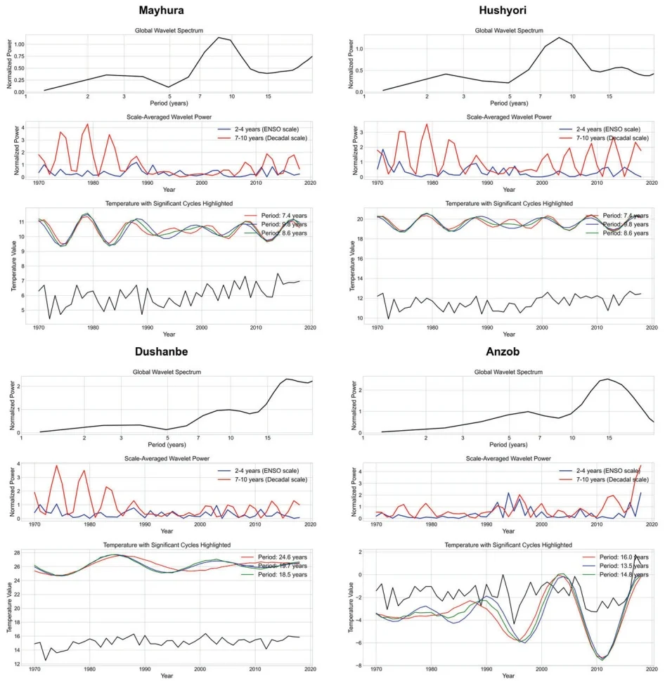
Fig. 16 Dominant periodicities of temperature data across all stations

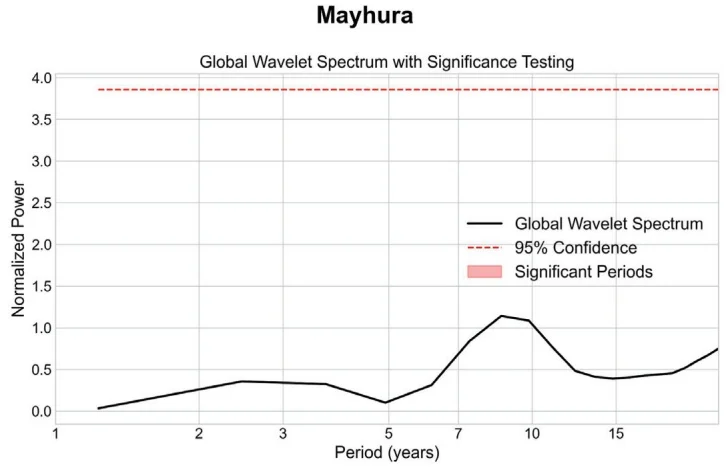
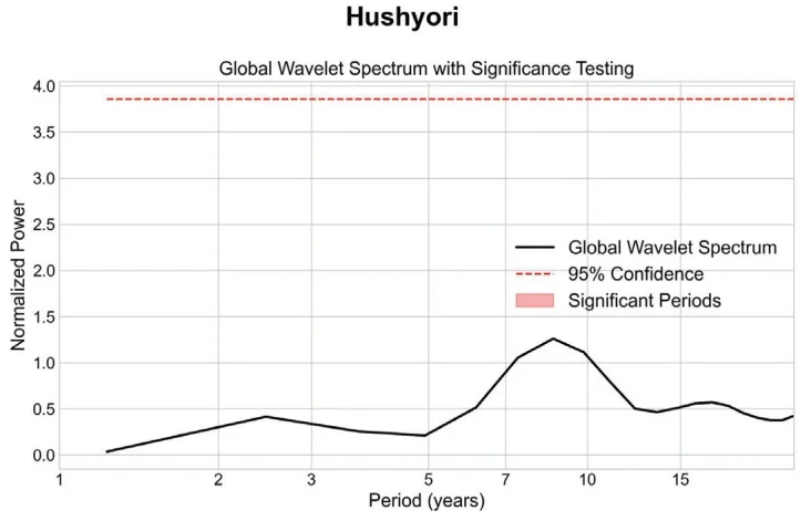
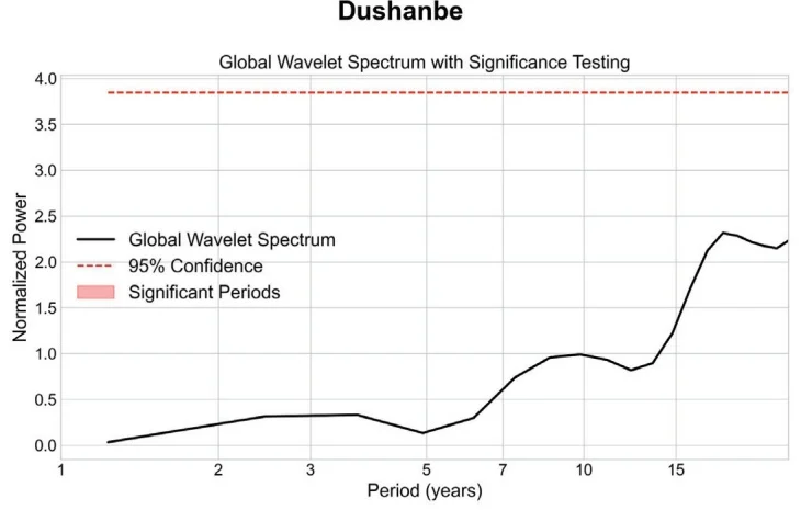
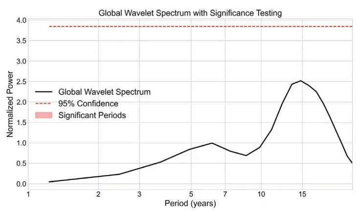
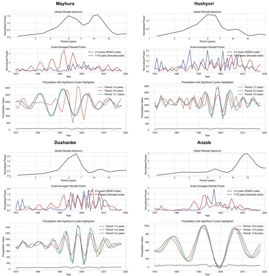
Fig. 18 Dominant periodicities of precipitation data across all stations

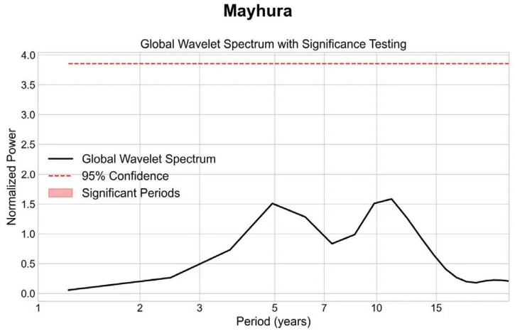
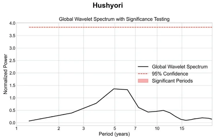
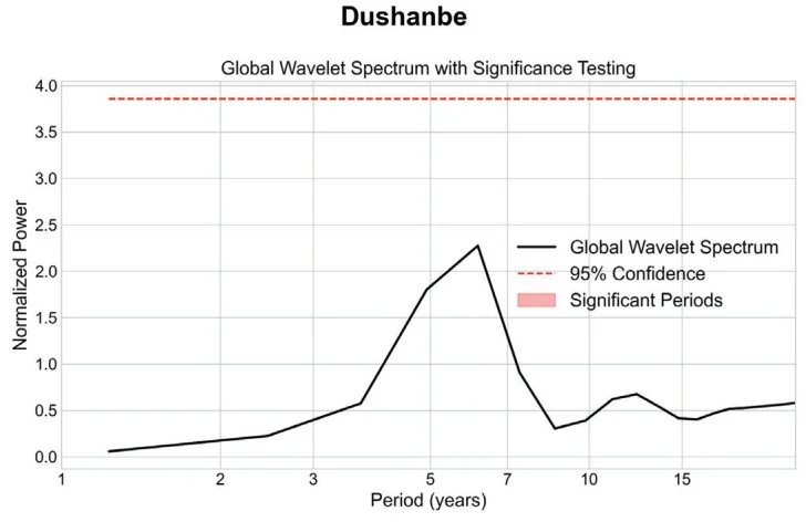
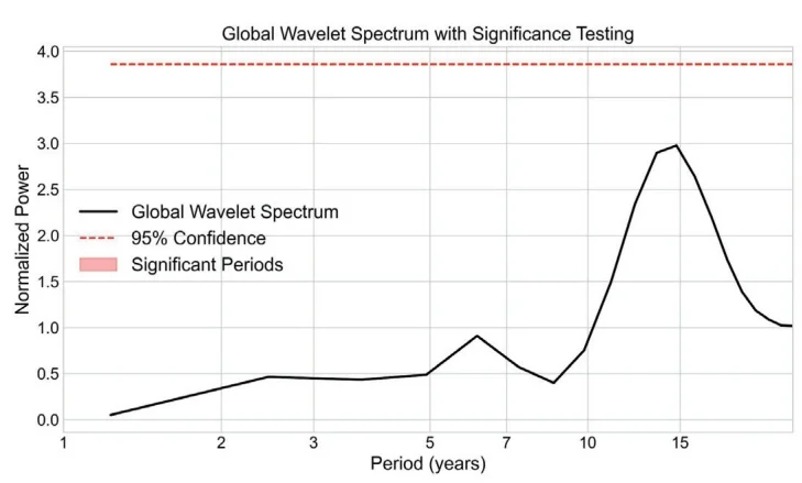
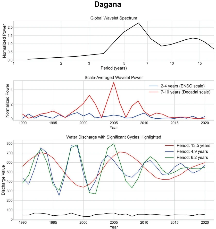
Fig. 20 Dominant periodicities of water discharge data at Dagana station

Dagana

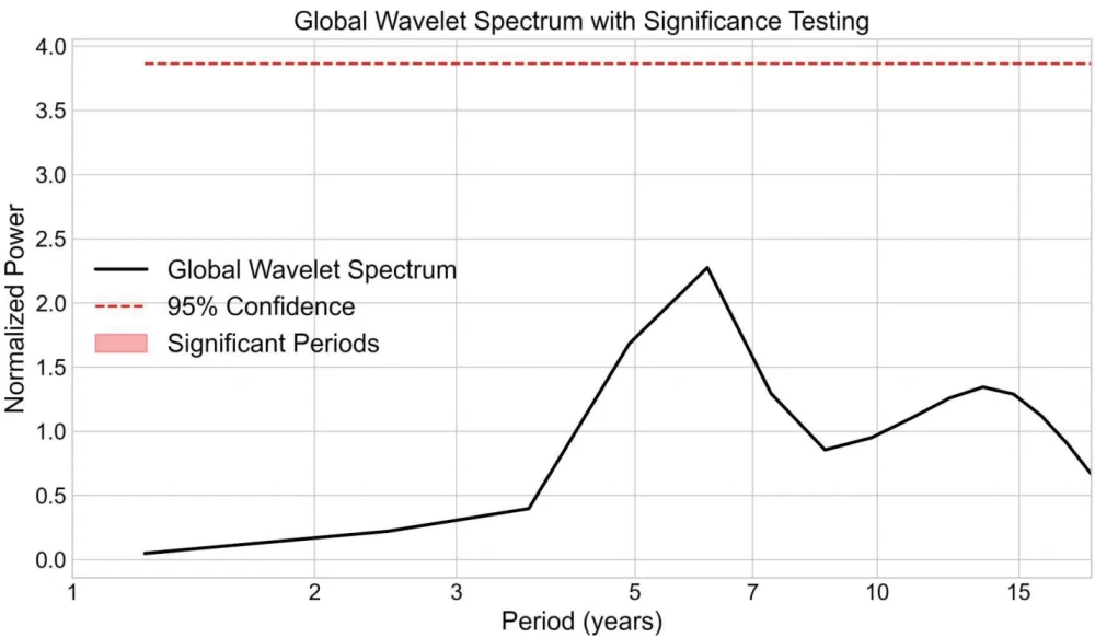
Fig. 21 Global wavelet spectrum with significance testing for Water discharge at Dagana station